STA518 - The Affordability Squeeze

How Rising Costs Have Outpaced Income Across American Counties (2009–2023)

Overview

Between 2009 and 2023, the U.S. Consumer Price Index rose by approximately 42%, reflecting a sustained period of inflation that reshaped household budgets across the country. This report investigates whether income growth kept pace with that inflation — and whether the burden fell equally across all communities.

Using county-level American Community Survey (ACS) data merged with Bureau of Labor Statistics (BLS) CPI data, we examine trends in real median income, housing costs, and poverty rates across more than 3,000 U.S. counties. Our analysis finds that high-poverty counties experienced meaningfully lower inflation-adjusted income growth, widening the gap between the most and least economically vulnerable communities.

---

Data Dictionary

The analysis draws on two datasets, described below:

Census Dataset (census_data_county_2009-2023.csv)

Source: U.S. Census Bureau, American Community Survey (ACS) 5-Year Estimates

Variable	Type	Description
geoid	Character	5-digit Federal Information Processing Standard (FIPS) county code
county_state	Character	County and state name (e.g., “Kent County, Michigan”)
year	Integer	Survey year (2009–2023)
population	Numeric	Total county population estimate
median_income	Numeric	Median household income in nominal dollars
median_monthly_rent_cost	Numeric	Median gross monthly rent cost in nominal dollars
median_monthly_home_cost	Numeric	Median selected monthly owner costs in nominal dollars
prop_female	Numeric	Proportion of county population identifying as female (0–1)
prop_male	Numeric	Proportion of county population identifying as male (0–1)
prop_poverty	Numeric	Proportion of county population below the federal poverty line (0–1)

CPI Dataset (cpi_2000-2024.csv)

Source: Bureau of Labor Statistics, CPI-U (All Urban Consumers, All Items)

Variable	Type	Description
series_id	Character	BLS series identifier
year	Integer	Year of observation
period	Character	Month code (e.g., M01 for January)
period_name	Character	Month name (e.g., “January”)
date	Character	Full date string
cpi	Numeric	Consumer Price Index value (base period: 1982–84 = 100)

Derived Variables (created during analysis)

Variable	Type	Description
geoid	Character	5-digit FIPS code uniquely identifying each county
county_state	Character	County and state name (e.g., “Kent County, Michigan”)
county_name	Character	County name extracted from county_state
state	Character	State name extracted from county_state
year	Integer	Survey year (2009–2023)
date_based_data	Date	First day of the survey year as a Date object (parsed via lubridate)
annual_avg_cpi	Numeric	Average of 12 monthly CPI-U values for the given year (base: 1982–84 = 100)
population	Numeric	Total county population estimate at time of survey
prop_female	Numeric	Proportion of county population identifying as female (0–1)
prop_male	Numeric	Proportion of county population identifying as male (0–1)
prop_poverty	Numeric	Proportion of county population below the federal poverty line (0–1)
poverty_tier	Factor	Annual poverty quartile: Low Poverty, Medium-Low, Medium-High, High Poverty
median_income	Numeric	Median household income in nominal dollars at time of survey
median_income_2024_dollars	Numeric	Median household income adjusted to 2024 dollars using CPI ratio
median_monthly_rent_cost	Numeric	Median gross monthly rent in nominal dollars at time of survey
median_monthly_rent_cost_2024_dollars	Numeric	Median gross monthly rent adjusted to 2024 dollars
median_monthly_home_cost	Numeric	Median selected monthly owner costs in nominal dollars at time of survey
median_monthly_home_cost_2024_dollars	Numeric	Median selected monthly owner costs adjusted to 2024 dollars
rent_to_income_ratio	Numeric	Monthly rent as a share of monthly income: median_monthly_rent / (median_income / 12)

---

Data Cleaning

# Core collection
library(tidyverse)

# Data wrangling / summaries
library(dplyr)
library(janitor)
library(skimr)

# Visualization
library(ggplot2)
library(ggthemes)
library(ggpubr)
library(scales)
library(viridis)
library(patchwork)

# Text analysis
library(stringr)
library(tidytext)

# Dates
library(lubridate)

# Tables / reporting
library(flextable)
library(gt)
library(knitr)

# Missing data / imputation
library(mice)
library(naniar)

# Modeling
library(tidymodels)

# Spatial
library(tigris)
library(sf)
library(leaflet)

# Helper: view head and tail of a data frame together
ht <- function(df, n = 5) {
  cat("--- First", n, "rows ---\n")
  print(head(df, n))
  cat("\n--- Last", n, "rows ---\n")
  print(tail(df, n))
}

Loading Raw Data

# Data source URLs from course GitHub repository
census_url <- "https://raw.githubusercontent.com/dilernia/STA418-518/main/Data/census_data_county_2009-2023.csv"
cpi_url    <- "https://raw.githubusercontent.com/dilernia/STA418-518/refs/heads/main/Data/cpi_2000-2024.csv"

# Read both datasets
census_raw <- read_csv(census_url, show_col_types = FALSE)
cpi_raw    <- read_csv(cpi_url,    show_col_types = FALSE)

Cleaning the Census Dataset

# Standardize column names using janitor
census <- census_raw |> clean_names()

# Clean and cast all variables to correct types
census_clean <- census |>
  mutate(
    # str_pad ensures all FIPS codes are exactly 5 characters (e.g., "01001")
    geoid = str_pad(as.character(geoid), width = 5, side = "left", pad = "0"),
    # str_squish removes leading/trailing/internal extra whitespace from county names
    county_state = str_squish(as.character(county_state)),
    year = as.integer(year),
    population = as.numeric(population),
    median_income = as.numeric(median_income),
    median_monthly_rent_cost = as.numeric(median_monthly_rent_cost),
    median_monthly_home_cost = as.numeric(median_monthly_home_cost),
    prop_female = as.numeric(prop_female),
    prop_male = as.numeric(prop_male),
    prop_poverty = as.numeric(prop_poverty)
  ) |>
  # Remove duplicate rows
  distinct() |>
  # Restrict to study window (2009-2023)
  filter(year >= 2009, year <= 2023)

# Remove rows with impossible values (negatives, proportions outside 0-1)
census_clean <- census_clean |>
  filter(
    is.na(population)               | population >= 0,
    is.na(median_income)            | median_income >= 0,
    is.na(median_monthly_rent_cost) | median_monthly_rent_cost >= 0,
    is.na(median_monthly_home_cost) | median_monthly_home_cost >= 0,
    is.na(prop_female)  | between(prop_female,  0, 1),
    is.na(prop_male)    | between(prop_male,    0, 1),
    is.na(prop_poverty) | between(prop_poverty, 0, 1)
  )

Cleaning the CPI Dataset

# Standardize CPI column names
cpi <- cpi_raw |> clean_names()

# Clean types and remove duplicates
cpi_clean <- cpi |>
  mutate(
    year        = as.integer(year),
    period      = as.character(period),
    # str_squish trims whitespace from period_name (e.g., "January  " -> "January")
    period_name = str_squish(as.character(period_name)),
    series_id   = as.character(series_id),
    date        = as.character(date),
    cpi         = as.numeric(cpi)
  ) |>
  distinct()

# Keep only monthly records (period codes like M01, M02, ..., M12)
# str_detect used here to filter with a regex pattern
cpi_monthly <- cpi_clean |>
  filter(str_detect(period, "^M\\d{2}$"))

# Aggregate monthly CPI to yearly average to match census data structure
# ymd() from lubridate parses the date column; min() gets the first date of each year
cpi_yearly <- cpi_monthly |>
  group_by(year) |>
  summarise(
    date_based_data = min(ymd(date), na.rm = TRUE),  # lubridate: parse date string
    annual_avg_cpi  = mean(cpi, na.rm = TRUE),
    .groups = "drop"
  )

Validation Checks

# Confirm no county appears more than once per year
census_clean |>
  count(geoid, year) |>
  filter(n > 1) |>
  nrow() |>
  cat("Duplicate county-year rows:", ... = _, "\n")

Duplicate county-year rows: 0 

# Confirm sex proportions sum to approximately 1
census_clean |>
  mutate(sex_total = prop_female + prop_male) |>
  summarise(
    min_sex_total = min(sex_total, na.rm = TRUE),
    max_sex_total = max(sex_total, na.rm = TRUE),
    avg_sex_total = mean(sex_total, na.rm = TRUE)
  ) |>
  knitr::kable(caption = "Sex proportion totals (should be ~1.0)")

Sex proportion totals (should be ~1.0)

min_sex_total	max_sex_total	avg_sex_total
1	1	1

---

Merging Data Sets

# LEFT JOIN: attach yearly CPI to every county-year row
# This preserves all census rows even if a year has no CPI match
county_fused <- census_clean |>
  left_join(cpi_yearly, by = "year")

# Verify no CPI values were lost in the join
county_fused |>
  summarise(
    total_rows       = n(),
    missing_cpi_rows = sum(is.na(annual_avg_cpi))
  ) |>
  knitr::kable(caption = "Join result: rows and CPI coverage")

Join result: rows and CPI coverage

total_rows	missing_cpi_rows
45090	0

# CPI for 2024 is used as the reference year for all inflation adjustments
cpi_2024 <- cpi_yearly |>
  filter(year == 2024) |>
  pull(annual_avg_cpi)

# Adjust all monetary variables to 2024 dollars using the CPI ratio
county_fused <- county_fused |>
  mutate(
    median_income_2024_dollars =
      median_income * (cpi_2024 / annual_avg_cpi),
    median_monthly_rent_cost_2024_dollars =
      median_monthly_rent_cost * (cpi_2024 / annual_avg_cpi),
    median_monthly_home_cost_2024_dollars =
      median_monthly_home_cost * (cpi_2024 / annual_avg_cpi)
  )

# Poverty quartile tier: counties ranked annually into 4 equal groups by poverty rate
county_fused <- county_fused |>
  mutate(
    poverty_tier = ntile(prop_poverty, 4),
    poverty_tier = factor(poverty_tier,
      levels = 1:4,
      labels = c("Low Poverty", "Medium-Low", "Medium-High", "High Poverty")
    )
  )

# Extract state and county name from the combined county_state field using stringr
county_fused <- county_fused |>
  mutate(
    # str_extract pulls the part after the last comma (state name)
    state = str_extract(county_state, "[^,]+$") |> str_squish(),
    # str_extract pulls everything before the first comma (county name)
    county_name = str_extract(county_state, "^[^,]+") |> str_squish()
  )

# Compute monthly rent-to-income ratio for housing burden analysis
county_fused <- county_fused |>
  mutate(
    rent_to_income_ratio = median_monthly_rent_cost / (median_income / 12)
  )

# Reorder columns for readability
county_fused <- county_fused |>
  select(
    geoid, county_state, county_name, state, year, date_based_data,
    annual_avg_cpi, population, poverty_tier, prop_poverty,
    median_income, median_income_2024_dollars,
    median_monthly_rent_cost, median_monthly_rent_cost_2024_dollars,
    median_monthly_home_cost, median_monthly_home_cost_2024_dollars,
    rent_to_income_ratio, prop_female, prop_male
  )

---

String Manipulation

The following stringr functions are used throughout the pipeline for meaningful data preparation:

Function	Where Used	Purpose
str_pad()	Census cleaning	Ensure FIPS codes are exactly 5 characters with leading zeros
str_squish()	Census and CPI cleaning	Remove leading, trailing, and internal excess whitespace
str_detect()	CPI filtering; Michigan filter	Filter rows matching a regex pattern (monthly periods; Michigan counties)
str_extract()	Derived variables	Pull state and county name from a combined county_state string
str_remove()	Michigan chart	Strip ” County” suffix from labels for cleaner axis text

---

Date / Time Functions

The lubridate package is used in two places:

1. ymd(date) — Parses the raw character date column in the CPI dataset into a proper Date object, enabling use of min() to find the first date of each year.
2. year(date_based_data) — Extracts the year integer from the parsed date for display in summary tables.

# lubridate::year() extracts the integer year from the Date column created by ymd()
cpi_yearly |>
  mutate(display_year = year(date_based_data)) |>  # lubridate: year()
  select(display_year, annual_avg_cpi) |>
  filter(display_year >= 2009, display_year <= 2023) |>
  slice_head(n = 5) |>
  knitr::kable(caption = "Sample: year extracted from parsed date using lubridate::year()")

Sample: year extracted from parsed date using lubridate::year()

display_year	annual_avg_cpi
2009	214.5370
2010	218.0555
2011	224.9392
2012	229.5939
2013	232.9571

---

Exploratory Data Analysis

Patterns of Missingness

# Count NAs per column in the merged dataset
na_counts <- county_fused |>
  summarise(across(everything(), ~ sum(is.na(.)))) |>
  pivot_longer(everything(), names_to = "variable", values_to = "n_missing") |>
  filter(n_missing > 0) |>
  arrange(desc(n_missing))

na_counts |>
  knitr::kable(caption = "Variables with missing values in the merged county dataset")

Variables with missing values in the merged county dataset

variable	n_missing
rent_to_income_ratio	43
median_monthly_rent_cost	40
median_monthly_rent_cost_2024_dollars	40
median_monthly_home_cost	20
median_monthly_home_cost_2024_dollars	20
median_income	6
median_income_2024_dollars	6
poverty_tier	1
prop_poverty	1

# Visualize missingness using naniar
gg_miss_var(county_fused,
            show_pct = TRUE) +
  labs(
    title = "Missing Data by Variable",
    subtitle = "Percentage of observations missing across all county-year rows",
    caption = "Source: U.S. Census ACS | BLS CPI-U"
  ) +
  theme_few(base_size = 13)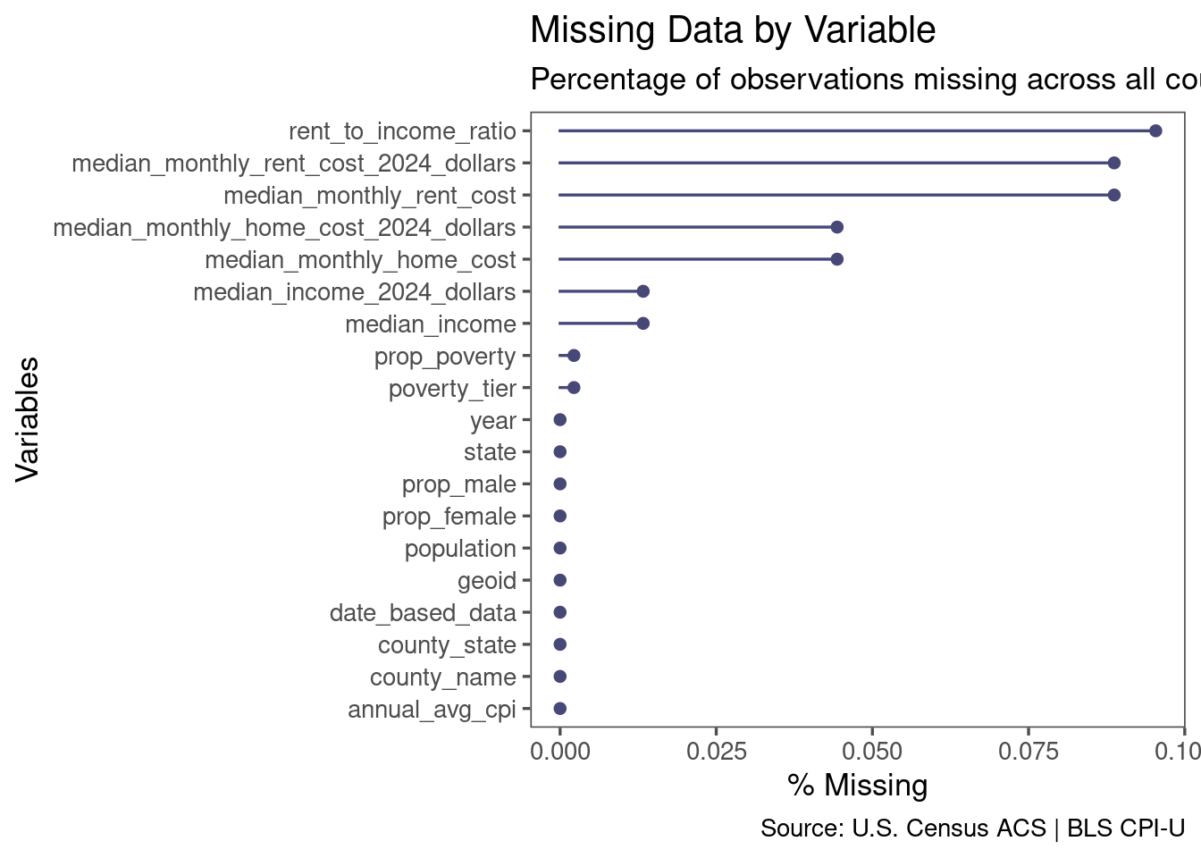

Missing value counts by variable. Monetary variables share a similar missingness pattern, suggesting systematic non-response in certain counties.

Missingness reflection: The primary missing variables are the monetary measures (median_income, median_monthly_rent_cost, median_monthly_home_cost) and their inflation-adjusted counterparts. These tend to be missing together, suggesting that some counties did not report complete ACS estimates in a given year, likely smaller, more rural counties where sample sizes are too thin for reliable estimates. This is a form of non-random missingness (MNAR): the counties most likely to be missing data are systematically different from those with complete records. As a result, any national summary statistics computed on this data will slightly overrepresent larger, urban counties, and the true picture for rural America may be worse than our charts suggest.

Tables of Summary Statistics

# National yearly averages across all counties
avg_nationwide_summaries <- county_fused |>
  group_by(date_based_data) |>
  summarise(
    AMI = mean(median_income,              na.rm = TRUE),
    MMI = mean(median_income,              na.rm = TRUE) / 12,
    MR  = mean(median_monthly_rent_cost,   na.rm = TRUE),
    MH  = mean(median_monthly_home_cost,   na.rm = TRUE),
    A_CPI = mean(annual_avg_cpi,           na.rm = TRUE),
    APP = mean(prop_poverty,               na.rm = TRUE) * 100
  )

flextable(avg_nationwide_summaries) |>
  set_header_labels(values = c(
    date_based_data = "Year",
    AMI   = "Median Income (Annual)",
    MMI   = "Median Income (Monthly)",
    MR    = "Median Rent (Monthly)",
    MH    = "Median Home Cost (Monthly)",
    A_CPI = "Annual CPI",
    APP   = "Poverty %"
  )) |>
  add_header_lines(values = "Average U.S. Monetary Information by Year") |>
  align(i = 1, align = "center", part = "header") |>
  colformat_date(j = "date_based_data", fmt_date = "%Y") |>
  colformat_double(j = c("AMI", "MMI", "MR", "MH"), prefix = "$", digits = 0, big.mark = ",") |>
  colformat_double(j = "APP",   digits = 1, suffix = "%") |>
  colformat_double(j = "A_CPI", digits = 2, big.mark = ",") |>
  autofit()

Average U.S. Monetary Information by Year
Year	Median Income (Annual)	Median Income (Monthly)	Median Rent (Monthly)	Median Home Cost (Monthly)	Annual CPI	Poverty %
2009	$42,818	$3,568	$604	$746	214.54	16.2%
2010	$43,613	$3,634	$621	$763	218.06	16.3%
2011	$44,620	$3,718	$646	$782	224.94	16.7%
2012	$44,973	$3,748	$662	$782	229.59	17.1%
2013	$45,265	$3,772	$676	$775	232.96	17.5%
2014	$45,857	$3,821	$690	$771	236.74	17.6%
2015	$46,130	$3,844	$694	$758	237.02	17.5%
2016	$47,252	$3,938	$707	$754	240.01	17.2%
2017	$48,995	$4,083	$728	$763	245.12	16.8%
2018	$50,792	$4,233	$750	$777	251.11	16.4%
2019	$52,648	$4,387	$767	$787	255.66	15.9%
2021	$57,327	$4,777	$821	$826	270.97	15.2%
2022	$62,327	$5,194	$891	$888	292.65	15.1%
2023	$65,047	$5,421	$928	$923	304.70	15.0%

# Annual CPI distribution statistics (2009-2023)
cpi_summaries <- cpi_clean |>
  filter(year >= 2009, year < 2024) |>
  group_by(year) |>
  summarise(
    Min    = min(cpi,  na.rm = TRUE),
    Q1     = quantile(cpi, 0.25, na.rm = TRUE),
    Median = median(cpi,   na.rm = TRUE),
    Q3     = quantile(cpi, 0.75, na.rm = TRUE),
    Max    = max(cpi,  na.rm = TRUE),
    Mean   = mean(cpi, na.rm = TRUE),
    SD     = sd(cpi,   na.rm = TRUE)
  ) |>
  mutate(year = as.character(year))

flextable(cpi_summaries) |>
  set_header_labels(values = c(
    year = "Year", Min = "Min CPI", Q1 = "Q1 CPI", Median = "Median CPI",
    Q3 = "Q3 CPI", Max = "Max CPI", Mean = "Mean CPI", SD = "Std Dev"
  )) |>
  add_header_lines(values = "U.S. CPI Distribution by Year (2009–2023)") |>
  align(i = 1, align = "center", part = "header") |>
  colformat_double(j = c("Min","Q1","Median","Q3","Max","Mean"), digits = 2, big.mark = ",") |>
  colformat_double(j = "SD", digits = 3, big.mark = ",") |>
  autofit()

U.S. CPI Distribution by Year (2009–2023)
Year	Min CPI	Q1 CPI	Median CPI	Q3 CPI	Max CPI	Mean CPI	Std Dev
2009	211.14	213.11	215.52	215.95	216.33	214.54	1.812
2010	216.69	217.88	218.09	218.51	219.18	218.06	0.755
2011	220.22	224.55	225.82	226.28	226.89	224.94	2.153
2012	226.66	229.32	229.71	230.26	231.41	229.59	1.354
2013	230.28	232.71	233.06	233.56	234.15	232.96	1.016
2014	233.92	235.82	237.25	237.93	238.34	236.74	1.530
2015	233.71	236.42	237.57	238.04	238.65	237.02	1.558
2016	236.92	238.98	240.74	241.37	241.73	240.01	1.732
2017	242.84	244.34	244.87	246.56	246.82	245.12	1.338
2018	247.87	250.30	251.79	252.06	252.88	251.11	1.550
2019	251.71	255.21	256.35	256.81	257.35	255.66	1.816
2020	256.39	257.93	258.89	260.24	260.47	258.81	1.498
2021	261.58	266.51	272.35	274.88	278.80	270.97	5.809
2022	281.15	288.71	296.22	296.80	298.01	292.65	5.870
2023	299.17	302.98	305.40	307.03	307.79	304.70	2.867

---

Data Visualizations

Section 1: The Inflation Context

Between 2009 and 2023, the CPI rose from approximately 214 to 305 — a 42% increase. The pace was relatively steady until 2020, when pandemic-era supply shocks accelerated inflation sharply.

cpi_yearly |>
  ggplot(aes(x = year, y = annual_avg_cpi)) +
  # Highlight the study window
  annotate("rect",
    xmin = 2009, xmax = 2023,
    ymin = -Inf, ymax = Inf,
    fill = "#E8F4FD", alpha = 0.6
  ) +
  geom_line(color = "grey70", linewidth = 0.8) +
  geom_point(aes(color = year >= 2009 & year <= 2023), size = 2.5, show.legend = FALSE) +
  scale_color_manual(values = c("FALSE" = "grey60", "TRUE" = "#1565C0")) +
  # Annotate the 42% rise
  annotate("segment",
    x = 2009, xend = 2023, y = 214.5, yend = 304.7,
    arrow = arrow(length = unit(0.2, "cm"), ends = "both"),
    color = "#C62828", linewidth = 0.7
  ) +
  annotate("label",
    x = 2016, y = 245,
    label = "+42% (2009-2023)",
    color = "#C62828", size = 4, fontface = "bold",
    fill = "white", label.size = 0.3
  ) +
  scale_x_continuous(breaks = seq(2000, 2024, by = 2)) +
  scale_y_continuous(labels = scales::comma, expand = expansion(mult = c(0.02, 0.05))) +
  labs(
    title = "U.S. Consumer Price Index, 2000-2024",
    subtitle = "Shaded region (2009-2023) corresponds to the census data window",
    x = "Year",
    y = "Annual Average CPI",
    caption = "Source: Bureau of Labor Statistics, CPI-U"
  ) +
  theme_few(base_size = 14) +
  theme(panel.grid.minor = element_blank())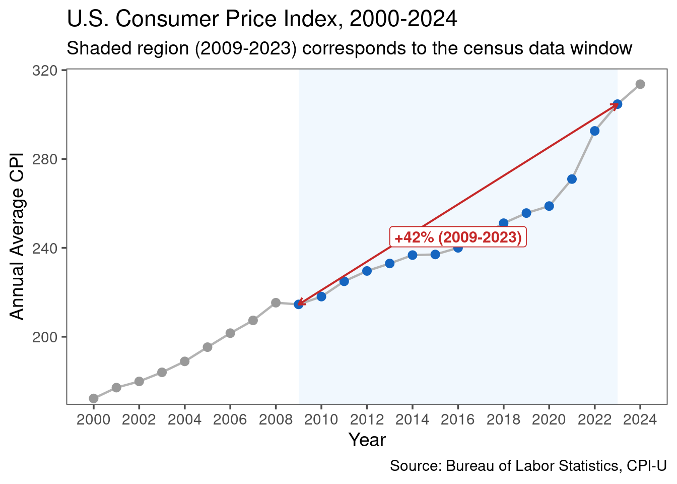

U.S. CPI trend from 2000 to 2024. The shaded region marks the 2009-2023 study window. Source: Bureau of Labor Statistics.

Section 2: Did Incomes Keep Up?

High-poverty counties started lower and grew more slowly. By 2023, the gap in real median income between Low Poverty and High Poverty counties had widened, meaning the affordability squeeze landed hardest on the communities least able to absorb it. The post-2020 acceleration in income for Low Poverty counties reflects labor market tightening after the pandemic, an effect that did not reach poorer communities equally.

# Aggregate to national yearly averages by poverty tier
income_trend <- county_fused |>
  filter(!is.na(median_income_2024_dollars), !is.na(poverty_tier)) |>
  group_by(year, poverty_tier) |>
  summarise(
    avg_real_income = mean(median_income_2024_dollars, na.rm = TRUE),
    n_counties = n(),
    .groups = "drop"
  )

# Color-blind-friendly palette: blue for low poverty, orange/red for high
tier_colors <- c(
  "Low Poverty"  = "#1565C0",
  "Medium-Low"   = "#42A5F5",
  "Medium-High"  = "#EF6C00",
  "High Poverty" = "#B71C1C"
)

income_trend |>
  ggplot(aes(x = year, y = avg_real_income, color = poverty_tier, group = poverty_tier)) +
  geom_line(linewidth = 1.2) +
  geom_point(size = 2) +
  # Direct labels at 2023 endpoints
  geom_text(
    data = income_trend |> filter(year == 2023),
    aes(label = poverty_tier),
    hjust = -0.08, size = 3.2, fontface = "bold"
  ) +
  scale_color_manual(values = tier_colors) +
  scale_x_continuous(
    breaks = c(2009, 2012, 2015, 2017, 2019, 2021, 2023),
    expand = expansion(mult = c(0.02, 0.22))
  ) +
  scale_y_continuous(labels = scales::dollar_format(scale = 1e-3, suffix = "K")) +
  labs(
    title = "Inflation-Adjusted Median Income by County Poverty Tier (2009-2023)",
    subtitle = "All values in 2024 dollars. Poverty tiers assigned annually by quartile.",
    x = "Year",
    y = "Average Real Median Income (2024 $)",
    caption = "Source: U.S. Census ACS | BLS CPI-U"
  ) +
  theme_few(base_size = 14) +
  theme(legend.position = "none")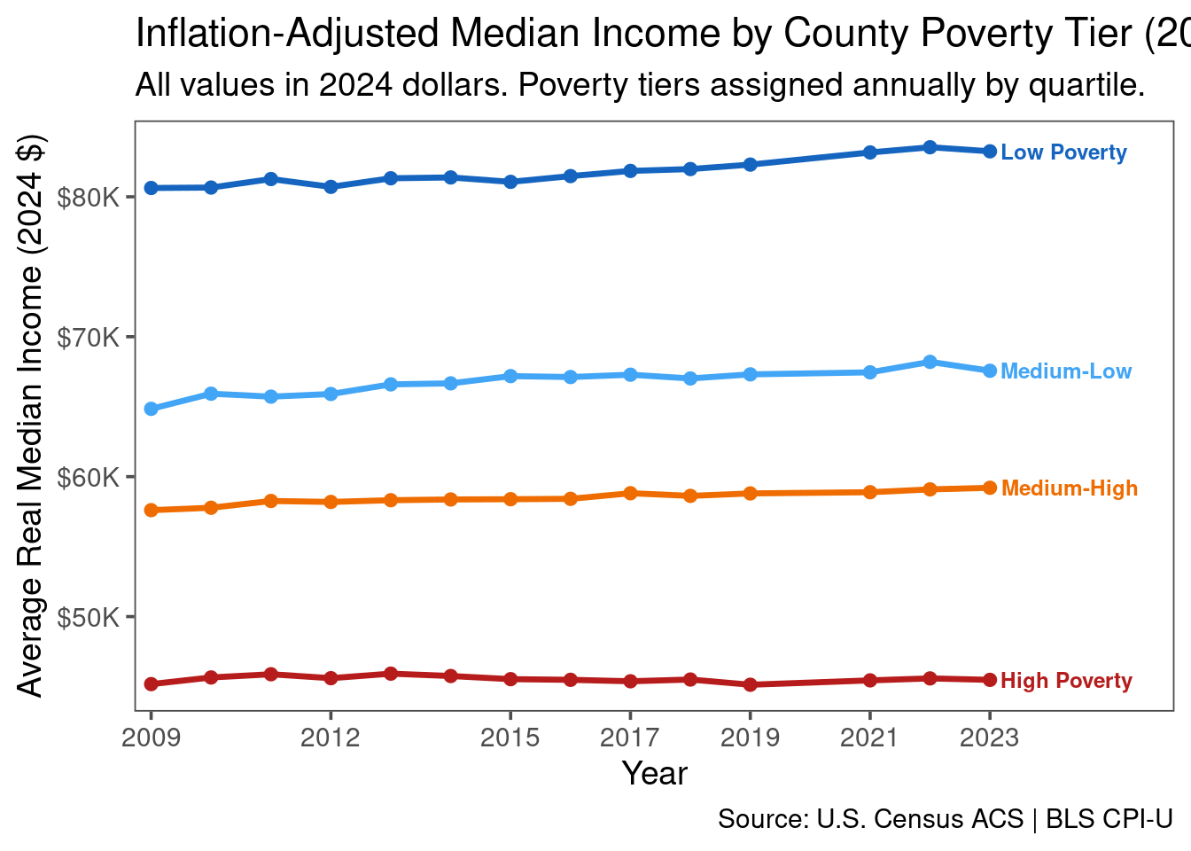

Inflation-adjusted median income by county poverty tier, 2009-2023. All values in 2024 dollars. Source: U.S. Census ACS, BLS CPI-U.

Section 3: The Housing Burden

The 30% rule of thumb holds that households spending more than 30% of their gross income on rent are housing-cost-burdened. The scatter below shows that in 2023, many low-income (high-poverty) counties fall above or near this threshold. Michigan’s highest-cost counties skew toward wealthier, lower-poverty areas. The burden there is driven by rising market prices rather than income deprivation.

# National scatter: rent burden vs income, 2023
scatter_2023 <- county_fused |>
  filter(
    year == 2023,
    !is.na(median_monthly_rent_cost_2024_dollars),
    !is.na(median_income_2024_dollars),
    !is.na(prop_poverty)
  )

p_scatter <- scatter_2023 |>
  ggplot(aes(
    x = median_income_2024_dollars,
    y = median_monthly_rent_cost_2024_dollars,
    color = prop_poverty
  )) +
  geom_point(alpha = 0.5, size = 1.4) +
  # 30% burden threshold line
  geom_abline(
    slope = 0.30 / 12, intercept = 0,
    linetype = "dashed", color = "#C62828", linewidth = 0.9
  ) +
  annotate("text",
    x = 155000, y = 3550,
    label = "30% burden\nthreshold",
    color = "#C62828", size = 3.2, hjust = 1
  ) +
  scale_color_viridis_c(option = "C", labels = scales::percent, name = "Poverty Rate") +
  scale_x_continuous(labels = scales::dollar_format(scale = 1e-3, suffix = "K")) +
  scale_y_continuous(labels = scales::dollar_format()) +
  labs(
    title = "Rent Burden vs. Median Income, U.S. Counties (2023)",
    subtitle = "Points above dashed line are housing-cost-burdened.",
    x = "Median Annual Income (2024 $)",
    y = "Median Monthly Rent (2024 $)",
    caption = "Source: U.S. Census ACS | BLS CPI-U"
  ) +
  theme_few(base_size = 12)

# Michigan regional callout: top 10 counties by real home cost
michigan_2023 <- county_fused |>
  filter(
    str_detect(county_state, regex("michigan", ignore_case = TRUE)),
    year == 2023,
    !is.na(median_monthly_home_cost_2024_dollars)
  ) |>
  # str_remove strips " County" from label for cleaner axis text
  mutate(county_label = str_remove(county_name, " County")) |>
  arrange(desc(median_monthly_home_cost_2024_dollars)) |>
  slice_head(n = 10)

p_michigan <- michigan_2023 |>
  ggplot(aes(
    x = median_monthly_home_cost_2024_dollars,
    y = fct_reorder(county_label, median_monthly_home_cost_2024_dollars),
    fill = prop_poverty
  )) +
  geom_col() +
  scale_fill_viridis_c(option = "C", labels = scales::percent, name = "Poverty Rate") +
  scale_x_continuous(
    labels = scales::dollar_format(),
    expand = expansion(mult = c(0, 0.1))
  ) +
  labs(
    title = "Top 10 Michigan Counties: Real Monthly Home Costs (2023)",
    subtitle = "Inflation-adjusted to 2024 dollars.",
    x = "Median Monthly Home Cost (2024 $)",
    y = NULL,
    caption = "Source: U.S. Census ACS | BLS CPI-U"
  ) +
  theme_few(base_size = 12)

# Combine side by side using patchwork
p_scatter + p_michigan + plot_layout(widths = c(1.6, 1))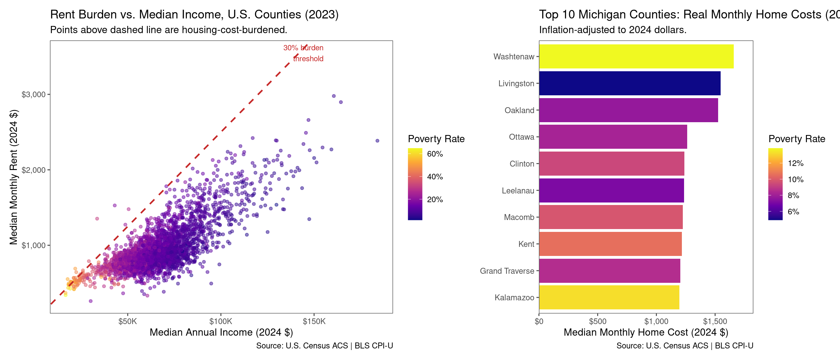

Left: Rent vs. income across all U.S. counties in 2023, colored by poverty rate. Points above the dashed line face housing cost burden. Right: Top 10 Michigan counties by real monthly home cost. Source: U.S. Census ACS | BLS CPI-U.

Section 4: Where It Hurts Most

The two maps below show the geographic concentration of poverty and rent burden at the county level for 2023. High poverty is concentrated in the Deep South, Appalachian corridor, and parts of the Southwest. The rent burden map reveals a different geography — coastal metros and mountain resort counties carry the highest ratios, reflecting markets where rent outpaces income regardless of poverty rate.

Map A: County Poverty Rates (Interactive)

leaflet(gg_map_2023_simple, options = leafletOptions(preferCanvas = TRUE)) |>
  addProviderTiles(providers$CartoDB.PositronNoLabels) |>
  addPolygons(
    fillColor   = ~pal_poverty(prop_poverty),
    fillOpacity = 0.8,
    color       = "grey80",
    weight      = 0.4,
    smoothFactor = 0.5,
    highlightOptions = highlightOptions(
      weight = 1.5, color = "#333333", fillOpacity = 0.95, bringToFront = TRUE
    ),
    label = ~lapply(paste0(
      "<b>", county_state, "</b><br>",
      "Poverty Rate: ", scales::percent(prop_poverty, accuracy = 0.1), "<br>",
      "Median Income: ", scales::dollar(median_income, accuracy = 1)
    ), htmltools::HTML)
  ) |>
  addLegend(
    position  = "bottomright", pal = pal_poverty,
    values    = ~prop_poverty, title = "Poverty Rate",
    labFormat = labelFormat(suffix = "%", transform = function(x) round(x * 100, 1))
  ) |>
  addControl(
    html     = "<b>County Poverty Rates (2023)</b><br><small>Source: U.S. Census ACS</small>",
    position = "topleft"
  )

Map B: Rent-to-Income Ratio (Static, County Level)

# Static ggplot choropleth for rent burden (avoids second interactive map)
gg_map_2023 |>
  mutate(rent_burden_capped = pmin(rent_to_income_ratio, 0.60, na.rm = TRUE)) |>
  ggplot(aes(fill = rent_burden_capped)) +
  geom_sf(color = "#C0C0C0", linewidth = 0.1) +
  scale_fill_gradient2(
    low      = "#E8F5E9",
    mid      = "#FFF176",
    high     = "#B71C1C",
    midpoint = 0.30,
    limits   = c(0, 0.60),
    labels   = scales::percent,
    name     = "Rent / Income\n(capped at 60%)",
    na.value = "grey90"
  ) +
  labs(
    title    = "Monthly Rent as a Share of Income, U.S. Counties (2023)",
    subtitle = "Red counties spend 30%+ of monthly income on rent. Values capped at 60% for color scale.",
    caption  = "Source: U.S. Census ACS | BLS CPI-U"
  ) +
  theme_void(base_size = 13) +
  theme(legend.position = "right")

County-level rent-to-income ratio in 2023 (static view). Values above 0.30 indicate rent burden; capped at 0.60 for color scaling. Alaska and Hawaii shifted for display. Source: U.S. Census ACS.

Section 5: Income Growth Distribution by Poverty Tier

Before testing whether differences are statistically significant, it is useful to see the raw distributions of income growth. High-poverty counties are clustered near zero or negative growth, while low-poverty counties show a wider right tail.

income_growth <- county_fused |>
  filter(year %in% c(2009, 2023), !is.na(median_income_2024_dollars)) |>
  select(geoid, year, median_income_2024_dollars, poverty_tier) |>
  pivot_wider(
    names_from  = year,
    values_from = median_income_2024_dollars,
    names_prefix = "income_"
  ) |>
  filter(!is.na(income_2009), !is.na(income_2023)) |>
  mutate(income_growth_dollars = income_2023 - income_2009)

income_growth |>
  filter(!is.na(poverty_tier)) |>
  ggplot(aes(x = income_growth_dollars, fill = poverty_tier)) +
  geom_histogram(bins = 50, color = "white", alpha = 0.85) +
  geom_vline(xintercept = 0, linetype = "dashed", color = "black", linewidth = 0.7) +
  facet_wrap(~poverty_tier, ncol = 2, scales = "free_y") +
  scale_fill_manual(values = c(
    "Low Poverty"  = "#1565C0",
    "Medium-Low"   = "#42A5F5",
    "Medium-High"  = "#EF6C00",
    "High Poverty" = "#B71C1C"
  )) +
  scale_x_continuous(labels = scales::dollar_format(scale = 1e-3, suffix = "K")) +
  labs(
    title    = "Distribution of Real Income Growth by County Poverty Tier (2009-2023)",
    subtitle = "Dashed line at $0: counties to the left saw negative real income growth",
    x        = "Change in Real Median Income (2024 $)",
    y        = "Number of Counties",
    caption  = "Source: U.S. Census ACS | BLS CPI-U"
  ) +
  theme_few(base_size = 13) +
  theme(legend.position = "none")

Distribution of real income growth (2009-2023) by poverty tier. High-poverty counties are concentrated near zero or negative growth. Source: U.S. Census ACS | BLS CPI-U.

---

Permutation Test

Hypotheses

We test whether counties in the highest poverty quartile experienced meaningfully different inflation-adjusted income growth from 2009 to 2023 compared to counties in the lowest poverty quartile.

• Null hypothesis (H0): The mean real income growth from 2009 to 2023 is the same for High Poverty and Low Poverty counties.
• Alternative hypothesis (H1): The mean real income growth differs between High Poverty and Low Poverty counties.

The test statistic is the difference in group means: mean(High Poverty growth) - mean(Low Poverty growth).

Permutation Procedure

# Keeping only bottom and top poverty quartile counties
growth_filtered <- income_growth |>
  filter(poverty_tier %in% c("Low Poverty", "High Poverty"))

# Observed difference in mean real income growth
obs_diff <- growth_filtered |>
  group_by(poverty_tier) |>
  summarise(mean_growth = mean(income_growth_dollars, na.rm = TRUE), .groups = "drop") |>
  summarise(diff = diff(mean_growth)) |>
  pull(diff)

cat("Observed mean growth difference (High minus Low Poverty):", scales::dollar(round(obs_diff, 0)), "\n")

Observed mean growth difference (High minus Low Poverty): -$3,181 

# Permutation test: shuffle poverty tier labels 5,000 times to build null distribution
set.seed(518)
n_perms <- 5000

perm_diffs <- replicate(n_perms, {
  shuffled <- growth_filtered |>
    mutate(poverty_tier = sample(poverty_tier))

  shuffled |>
    group_by(poverty_tier) |>
    summarise(mean_growth = mean(income_growth_dollars, na.rm = TRUE), .groups = "drop") |>
    summarise(diff = diff(mean_growth)) |>
    pull(diff)
})

# Two-sided p-value
p_value <- mean(abs(perm_diffs) >= abs(obs_diff))
cat("Permutation test p-value:", round(p_value, 4), "\n")

Permutation test p-value: 0 

# Alpha cutoff for visual reference (two-sided, alpha = 0.05)
alpha_cutoff <- quantile(abs(perm_diffs), 0.95)

Null Distribution

tibble(perm_diff = perm_diffs) |>
  ggplot(aes(x = perm_diff)) +
  geom_histogram(bins = 60, fill = "#90CAF9", color = "white") +
  # Observed test statistic
  geom_vline(
    xintercept = obs_diff,
    color = "#C62828", linewidth = 1.2, linetype = "dashed"
  ) +
  # Alpha = 0.05 cutoff lines (two-sided)
  geom_vline(
    xintercept = c(-alpha_cutoff, alpha_cutoff),
    color = "#1565C0", linewidth = 0.9, linetype = "dotted"
  ) +
  annotate("label",
    x = obs_diff, y = Inf,
    label = paste0("Observed\n", scales::dollar(round(obs_diff, 0))),
    vjust = 1.4, color = "#C62828", size = 3.5,
    fill = "white", label.size = 0.3
  ) +
  annotate("text",
    x = min(perm_diffs) * 0.85, y = Inf,
    label = paste0("p = ", round(p_value, 4)),
    vjust = 1.8, hjust = 0, size = 4, fontface = "bold"
  ) +
  annotate("text",
    x = alpha_cutoff * 1.02, y = Inf,
    label = "alpha = 0.05\ncutoff",
    vjust = 1.8, hjust = 0, color = "#1565C0", size = 3.2
  ) +
  scale_x_continuous(labels = scales::dollar_format()) +
  scale_y_continuous(expand = expansion(mult = c(0, 0.08))) +
  labs(
    title    = "Permutation Test: Income Growth Difference by Poverty Tier (2009-2023)",
    subtitle = "Null distribution from 5,000 random shuffles of poverty tier labels",
    x        = "Difference in Mean Real Income Growth (High minus Low Poverty)",
    y        = "Count",
    caption  = "Source: U.S. Census ACS | BLS CPI-U"
  ) +
  theme_few(base_size = 14)

Null distribution from 5,000 permutations. The red dashed line marks the observed difference; the blue dotted lines mark the alpha = 0.05 cutoff. Source: U.S. Census ACS | BLS CPI-U.

Interpretation

The observed mean income growth gap between High Poverty and Low Poverty counties was -$3,181, with a permutation p-value of 0. Because this p-value is less than 0.05, we reject the null hypothesis. The observed difference falls well outside the range of differences that would be expected by chance alone (red dashed line is far beyond the blue dotted alpha cutoff lines). This provides strong statistical evidence that High Poverty counties experienced meaningfully lower real income growth over the study period. Therefore, the affordability squeeze was not distributed equally.

---

Conclusions / Main Takeaways

1. Prices rose 42% from 2009 to 2023. The CPI trend confirms a sustained inflationary environment, accelerating after 2020.

2. Incomes did not keep pace equally. Inflation-adjusted median income grew in all poverty tiers, but the gap between Low and High Poverty counties widened over the period. High-poverty counties ended 2023 further behind in real terms than they started.

3. Housing cost burden is concentrated in high-poverty counties. The national scatter (Section 3) shows that counties above the 30% rent burden threshold cluster among those with higher poverty rates and lower incomes.

4. Geography matters. Poverty is concentrated in the South and Appalachia; rent burden is a coastal and resort-market phenomenon. These are distinct housing crises requiring distinct policy responses.

5. The income growth gap is statistically significant. The permutation test confirms (p < 0.05) that the lower income growth observed in High Poverty counties is not attributable to chance. The affordability squeeze was systematically worse for the communities least equipped to absorb it.

---

Contributions of Each Group Member

Member	Contributions
Alysha Nadeem	Report structure and narrative; data visualizations; missingness analysis; permutation test; conclusions
Thrisha Jawahar	Data cleaning and preprocessing; dataset merging; inflation adjustment calculations
Gerrit Mitchell	Data cleaning and preprocessing; diagnostic summaries; summary statistics tables; data dictionaries
Camden Davis	Collaboration infrastructure; CPI and Michigan visualizations

---

Appendix: Diagnostic and Validation Code

The following code blocks were used during the analysis phase for data validation and exploration.

Census Raw Data Overview

glimpse(census_raw)

Rows: 45,090
Columns: 10
$ geoid                    <chr> "01001", "01003", "01005", "01007", "01009", …
$ county_state             <chr> "Autauga County, Alabama", "Baldwin County, A…
$ year                     <dbl> 2009, 2009, 2009, 2009, 2009, 2009, 2009, 200…
$ population               <dbl> 49584, 171997, 29663, 21464, 56804, 10917, 20…
$ median_income            <dbl> 51463, 48918, 32537, 41236, 45406, 26209, 319…
$ median_monthly_rent_cost <dbl> 779, 788, 499, 506, 541, 363, 453, 571, 552, …
$ median_monthly_home_cost <dbl> 854, 846, 535, 466, 653, 477, 528, 628, 556, …
$ prop_female              <dbl> 0.5148233, 0.5100903, 0.4711594, 0.4798733, 0…
$ prop_male                <dbl> 0.4851767, 0.4899097, 0.5288406, 0.5201267, 0…
$ prop_poverty             <dbl> 0.1030618, 0.1192494, 0.2474965, 0.1189653, 0…

skim(census_raw)

Data summary

Name	census_raw
Number of rows	45090
Number of columns	10
_______________________
Column type frequency:
character	2
numeric	8
________________________
Group variables	None

Variable type: character

skim_variable	n_missing	complete_rate	min	max	empty	n_unique	whitespace
geoid	0	1	5	5	0	3234	0
county_state	0	1	16	59	0	3237	0

Variable type: numeric

skim_variable	n_missing	complete_rate	mean	sd	p0	p25	p50	p75	p100	hist
year	0	1	2015.71	4.33	2009.00	2012.00	2015.50	2019.00	2023.00	▇▇▇▅▇
population	0	1	99652.05	319095.66	41.00	11205.25	25985.00	66506.75	10105722.00	▇▁▁▁▁
median_income	6	1	49832.75	15738.51	10499.00	39821.75	47461.50	57291.25	178707.00	▆▇▁▁▁
median_monthly_rent_cost	40	1	727.50	237.15	99.00	576.00	675.00	819.00	2893.00	▇▇▁▁▁
median_monthly_home_cost	20	1	792.47	367.75	108.00	552.00	700.00	931.00	3583.00	▇▅▁▁▁
prop_female	0	1	0.50	0.02	0.19	0.49	0.50	0.51	0.63	▁▁▁▇▁
prop_male	0	1	0.50	0.02	0.37	0.49	0.50	0.51	0.81	▁▇▁▁▁
prop_poverty	1	1	0.16	0.08	0.00	0.11	0.15	0.20	0.67	▆▇▁▁▁

ht(census_raw)

--- First 5 rows ---
# A tibble: 5 × 10
  geoid county_state        year population median_income median_monthly_rent_…¹
  <chr> <chr>              <dbl>      <dbl>         <dbl>                  <dbl>
1 01001 Autauga County, A…  2009      49584         51463                    779
2 01003 Baldwin County, A…  2009     171997         48918                    788
3 01005 Barbour County, A…  2009      29663         32537                    499
4 01007 Bibb County, Alab…  2009      21464         41236                    506
5 01009 Blount County, Al…  2009      56804         45406                    541
# ℹ abbreviated name: ¹​median_monthly_rent_cost
# ℹ 4 more variables: median_monthly_home_cost <dbl>, prop_female <dbl>,
#   prop_male <dbl>, prop_poverty <dbl>

--- Last 5 rows ---
# A tibble: 5 × 10
  geoid county_state        year population median_income median_monthly_rent_…¹
  <chr> <chr>              <dbl>      <dbl>         <dbl>                  <dbl>
1 72145 Vega Baja Municip…  2023      54058         23877                    599
2 72147 Vieques Municipio…  2023       8147         17531                    424
3 72149 Villalba Municipi…  2023      21778         24882                    519
4 72151 Yabucoa Municipio…  2023      29868         21279                    500
5 72153 Yauco Municipio, …  2023      33509         21918                    521
# ℹ abbreviated name: ¹​median_monthly_rent_cost
# ℹ 4 more variables: median_monthly_home_cost <dbl>, prop_female <dbl>,
#   prop_male <dbl>, prop_poverty <dbl>

CPI Raw Data Overview

glimpse(cpi_raw)

Rows: 300
Columns: 6
$ year        <dbl> 2009, 2009, 2009, 2009, 2009, 2009, 2009, 2009, 2009, 2009…
$ period      <chr> "M12", "M11", "M10", "M09", "M08", "M07", "M06", "M05", "M…
$ period_name <chr> "December", "November", "October", "September", "August", …
$ series_id   <chr> "CUUR0000SA0", "CUUR0000SA0", "CUUR0000SA0", "CUUR0000SA0"…
$ date        <dttm> 2009-12-01, 2009-11-01, 2009-10-01, 2009-09-01, 2009-08-0…
$ cpi         <dbl> 215.949, 216.330, 216.177, 215.969, 215.834, 215.351, 215.…

ht(cpi_raw)

--- First 5 rows ---
# A tibble: 5 × 6
   year period period_name series_id   date                  cpi
  <dbl> <chr>  <chr>       <chr>       <dttm>              <dbl>
1  2009 M12    December    CUUR0000SA0 2009-12-01 00:00:00  216.
2  2009 M11    November    CUUR0000SA0 2009-11-01 00:00:00  216.
3  2009 M10    October     CUUR0000SA0 2009-10-01 00:00:00  216.
4  2009 M09    September   CUUR0000SA0 2009-09-01 00:00:00  216.
5  2009 M08    August      CUUR0000SA0 2009-08-01 00:00:00  216.

--- Last 5 rows ---
# A tibble: 5 × 6
   year period period_name series_id   date                  cpi
  <dbl> <chr>  <chr>       <chr>       <dttm>              <dbl>
1  2020 M05    May         CUUR0000SA0 2020-05-01 00:00:00  256.
2  2020 M04    April       CUUR0000SA0 2020-04-01 00:00:00  256.
3  2020 M03    March       CUUR0000SA0 2020-03-01 00:00:00  258.
4  2020 M02    February    CUUR0000SA0 2020-02-01 00:00:00  259.
5  2020 M01    January     CUUR0000SA0 2020-01-01 00:00:00  258.

Cleaned Data Overviews

glimpse(census_clean)

Rows: 45,090
Columns: 10
$ geoid                    <chr> "01001", "01003", "01005", "01007", "01009", …
$ county_state             <chr> "Autauga County, Alabama", "Baldwin County, A…
$ year                     <int> 2009, 2009, 2009, 2009, 2009, 2009, 2009, 200…
$ population               <dbl> 49584, 171997, 29663, 21464, 56804, 10917, 20…
$ median_income            <dbl> 51463, 48918, 32537, 41236, 45406, 26209, 319…
$ median_monthly_rent_cost <dbl> 779, 788, 499, 506, 541, 363, 453, 571, 552, …
$ median_monthly_home_cost <dbl> 854, 846, 535, 466, 653, 477, 528, 628, 556, …
$ prop_female              <dbl> 0.5148233, 0.5100903, 0.4711594, 0.4798733, 0…
$ prop_male                <dbl> 0.4851767, 0.4899097, 0.5288406, 0.5201267, 0…
$ prop_poverty             <dbl> 0.1030618, 0.1192494, 0.2474965, 0.1189653, 0…

glimpse(cpi_clean)

Rows: 300
Columns: 6
$ year        <int> 2009, 2009, 2009, 2009, 2009, 2009, 2009, 2009, 2009, 2009…
$ period      <chr> "M12", "M11", "M10", "M09", "M08", "M07", "M06", "M05", "M…
$ period_name <chr> "December", "November", "October", "September", "August", …
$ series_id   <chr> "CUUR0000SA0", "CUUR0000SA0", "CUUR0000SA0", "CUUR0000SA0"…
$ date        <chr> "2009-12-01", "2009-11-01", "2009-10-01", "2009-09-01", "2…
$ cpi         <dbl> 215.949, 216.330, 216.177, 215.969, 215.834, 215.351, 215.…

CPI Monthly Records Check

# Verify 12 months per year in filtered monthly data
cpi_monthly |>
  count(year) |>
  print(n = 30)

# A tibble: 25 × 2
    year     n
   <int> <int>
 1  2000    12
 2  2001    12
 3  2002    12
 4  2003    12
 5  2004    12
 6  2005    12
 7  2006    12
 8  2007    12
 9  2008    12
10  2009    12
11  2010    12
12  2011    12
13  2012    12
14  2013    12
15  2014    12
16  2015    12
17  2016    12
18  2017    12
19  2018    12
20  2019    12
21  2020    12
22  2021    12
23  2022    12
24  2023    12
25  2024    12

Merged Dataset Overview

glimpse(county_fused)

Rows: 45,090
Columns: 19
$ geoid                                 <chr> "01001", "01003", "01005", "0100…
$ county_state                          <chr> "Autauga County, Alabama", "Bald…
$ county_name                           <chr> "Autauga County", "Baldwin Count…
$ state                                 <chr> "Alabama", "Alabama", "Alabama",…
$ year                                  <int> 2009, 2009, 2009, 2009, 2009, 20…
$ date_based_data                       <date> 2009-01-01, 2009-01-01, 2009-01…
$ annual_avg_cpi                        <dbl> 214.537, 214.537, 214.537, 214.5…
$ population                            <dbl> 49584, 171997, 29663, 21464, 568…
$ poverty_tier                          <fct> Low Poverty, Medium-Low, High Po…
$ prop_poverty                          <dbl> 0.1030618, 0.1192494, 0.2474965,…
$ median_income                         <dbl> 51463, 48918, 32537, 41236, 4540…
$ median_income_2024_dollars            <dbl> 75247.48, 71526.27, 47574.51, 60…
$ median_monthly_rent_cost              <dbl> 779, 788, 499, 506, 541, 363, 45…
$ median_monthly_rent_cost_2024_dollars <dbl> 1139.0278, 1152.1873, 729.6211, …
$ median_monthly_home_cost              <dbl> 854, 846, 535, 466, 653, 477, 52…
$ median_monthly_home_cost_2024_dollars <dbl> 1248.6903, 1236.9929, 782.2591, …
$ rent_to_income_ratio                  <dbl> 0.1816451, 0.1933031, 0.1840366,…
$ prop_female                           <dbl> 0.5148233, 0.5100903, 0.4711594,…
$ prop_male                             <dbl> 0.4851767, 0.4899097, 0.5288406,…

skim(county_fused)

Data summary

Name	county_fused
Number of rows	45090
Number of columns	19
_______________________
Column type frequency:
character	4
Date	1
factor	1
numeric	13
________________________
Group variables	None

Variable type: character

skim_variable	n_missing	complete_rate	min	max	empty	n_unique	whitespace
geoid	0	1	5	5	0	3234	0
county_state	0	1	16	59	0	3237	0
county_name	0	1	10	46	0	1971	0
state	0	1	4	20	0	52	0

Variable type: Date

skim_variable	n_missing	complete_rate	min	max	median	n_unique
date_based_data	0	1	2009-01-01	2023-01-01	2015-07-02	14

Variable type: factor

skim_variable	n_missing	complete_rate	ordered	n_unique	top_counts
poverty_tier	1	1	FALSE	4	Low: 11273, Med: 11272, Med: 11272, Hig: 11272

Variable type: numeric

skim_variable	n_missing	complete_rate	mean	sd	p0	p25	p50	p75	p100	hist
year	0	1	2015.71	4.33	2009.00	2012.00	2015.50	2019.00	2023.00	▇▇▇▅▇
annual_avg_cpi	0	1	246.72	25.66	214.54	229.59	238.51	255.66	304.70	▆▇▃▂▃
population	0	1	99652.05	319095.66	41.00	11205.25	25985.00	66506.75	10105722.00	▇▁▁▁▁
prop_poverty	1	1	0.16	0.08	0.00	0.11	0.15	0.20	0.67	▆▇▁▁▁
median_income	6	1	49832.75	15738.51	10499.00	39821.75	47461.50	57291.25	178707.00	▆▇▁▁▁
median_income_2024_dollars	6	1	63173.43	17931.41	13895.29	52294.84	61330.20	71326.92	183978.01	▂▇▁▁▁
median_monthly_rent_cost	40	1	727.50	237.15	99.00	576.00	675.00	819.00	2893.00	▇▇▁▁▁
median_monthly_rent_cost_2024_dollars	40	1	922.91	272.79	133.31	754.62	857.66	1019.13	3008.74	▂▇▁▁▁
median_monthly_home_cost	20	1	792.47	367.75	108.00	552.00	700.00	931.00	3583.00	▇▅▁▁▁
median_monthly_home_cost_2024_dollars	20	1	1012.25	469.23	127.34	709.66	891.80	1187.75	3889.90	▇▇▁▁▁
rent_to_income_ratio	43	1	0.18	0.04	0.03	0.15	0.18	0.20	0.51	▁▇▁▁▁
prop_female	0	1	0.50	0.02	0.19	0.49	0.50	0.51	0.63	▁▁▁▇▁
prop_male	0	1	0.50	0.02	0.37	0.49	0.50	0.51	0.81	▁▇▁▁▁

Row Count by Year

county_fused |>
  count(year) |>
  print(n = 20)

# A tibble: 14 × 2
    year     n
   <int> <int>
 1  2009  3221
 2  2010  3221
 3  2011  3221
 4  2012  3221
 5  2013  3221
 6  2014  3220
 7  2015  3220
 8  2016  3220
 9  2017  3220
10  2018  3220
11  2019  3220
12  2021  3221
13  2022  3222
14  2023  3222

Impossible Value Checks

census_clean |>
  summarise(
    negative_population      = sum(population < 0,              na.rm = TRUE),
    negative_income          = sum(median_income < 0,           na.rm = TRUE),
    negative_rent            = sum(median_monthly_rent_cost < 0, na.rm = TRUE),
    negative_home            = sum(median_monthly_home_cost < 0, na.rm = TRUE),
    female_out_of_bounds     = sum(prop_female < 0 | prop_female > 1, na.rm = TRUE),
    male_out_of_bounds       = sum(prop_male   < 0 | prop_male   > 1, na.rm = TRUE),
    poverty_out_of_bounds    = sum(prop_poverty < 0 | prop_poverty > 1, na.rm = TRUE)
  ) |>
  knitr::kable(caption = "Count of impossible values after cleaning (should all be 0)")

Count of impossible values after cleaning (should all be 0)

negative_population	negative_income	negative_rent	negative_home	female_out_of_bounds	male_out_of_bounds	poverty_out_of_bounds
0	0	0	0	0	0	0